
Statistical models and likelihood
Stat 221, Lecture 6
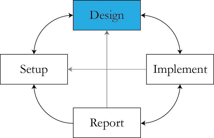
Lecture plan
- Design phase: what matters.
- R- and design-friendly ways to write the model.
- Actors in the model.
- Critiquing the modeling process.
Statistical models
- What do they mean to us as data analysts?
Doing things with models
- Formulating intuition.
- Answering a question.
- Checking goodness.
- Predicting.
- Generalizing.
Practical steps
- Formulate questions \\( \rightarrow \\) benchmarks to check against.
- Model "mean response".
- Model noise around it.
- Incorporate features of the system.
$$Y \sim f_{\theta}(X, \epsilon)$$
Classic example - regression
$$\vec{Y} \sim \mathbf{X}\vec{\beta} + \vec{\epsilon}, \rr{ } \vec{\epsilon} \sim N\left(0, \sigma^2\mathbf{I}\right)$$
- or
$$\begin{align}Y_i & \sim \beta_0 + X_1\beta_1 + \ldots + X_n\beta_n + \epsilon_i \\ \epsilon_i & \sim N\left(0, \sigma^2\right)\end{align}$$
- or
$$\vec{Y} \sim N\left(\mathbf{X}\vec{\beta}, \sigma^2\mathbf{I}\right)$$
Data density (likelihood!)
$$f(y \given \theta, X)\, = \frac{1}{(2\pi \sigma^2)^{n/2}} e^{-\frac{1}{2\sigma^2}(y -X\beta)^T(y- X\beta)}$$
Alternatively, $$f(y \given \theta, X) = \prod_{i=1}^n \frac{1}{\sqrt{2\pi\sigma^2}} e^{\frac{1}{2\sigma^2} \left( y_i - (\beta_0 + x_1 \beta_1 + \ldots + x_p \beta_p)\right)^2}$$
Useful: matrix calculus.
Actors in the model
- Response.
- Covariates.
- Free parameters.
- Constants (numbers).
- Latent variables/missing data.
Example: AP model
$$$$\begin{align} Y_i \given Y_{r(i)} & \sim N \left(\rho Y_{r(i)} + (1 - \rho) \mu, (1 - \rho^2) \sigma^2 \right), \\Y_i & \sim N\left( \mu, \sigma^2 \right) \rr{ if } r(i)\rr{ doesn't exist}\end{align}$$$$
- You don't necessarily need covariates.
- Autoregressive flavor.
- Homophily intuition.
Data density
$$\begin{align}f(y \given \theta) = \prod_{i=1}^n & \frac{1}{\sqrt{2\pi\sigma^2(1 - \rho_i)^2}} \\ & e^{\frac{1}{2\sigma^2(1-\rho_i^2)}\left( y_i - \left( \rho_i y_{r(i)} + (1 - \rho_i) \mu\right)\right)}\end{align}$$
- \\(\rho_i = \begin{cases} \rho & \rr{if } i \rr{ is referred} \\ 0 & \rr{if } i \rr{ is a seed}\end{cases}\\)
R-friendly math
- Reduce the number of math symbols in your formulas.
- Use matrices and vectors.
- More on that later.
Generalizing the model
$$\begin{align}f(y \given \theta) = \prod_{i=1}^n & \frac{1}{\sqrt{2\pi\sigma^2(1 - \rho_i)^2}} \\ & e^{\frac{1}{2\sigma^2(1-\rho_i^2)}\left( y_i - \left( \rho_i y_{r(i)} + (1 - \rho_i) \mu\right)\right)}\end{align}$$
- \\(\rho_i = \begin{cases} \rho^{(1)} & \rr{if } i \rr{ is referred by close friend} \\ \rho^{(2)} & \rr{if } i \rr{ is referred by distant friend}\\ 0 & \rr{if } i \rr{ is a seed}\end{cases}\\)
Being creative
Switching actors around:
- Data augmentation - introducing latent variables.
- Free parameters can become latent variables.
- Constants can morph into parameters.
Constraining
- Domains and more involved constraints.
- Priors.
Beware of possible consequences:
- Effect on the estimand.
- Computing.
Other models
Probit regression $$Y_i \given Z_i = \begin{cases}1 \rr{ if } Z_i < X_i \beta \\ 0 \rr{ otherwise}\end{cases} , \rr{ } Z_i \sim N(0,1)$$
or $$Y_i \sim \rr{Bernoulli}\left(\Phi(X_i\beta) \right) $$
Data pmf
$$p(y \given \beta, X) \propto \prod_{i=1}^n \Phi(X_i \beta)^{y_i} \left( 1 - \Phi(X_i\beta)\right)^{y_i}$$
Hidden Markov Model
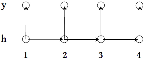
- \\(\{h_1, h_2, \ldots \} \\) live on discrete space, follow a Markov Process with a transition matrix \\( T_\theta \\).
- At time \\( t\\), state \\( h_t \\) emits observation \\( y_t \\) according to some specified model.
Data generation process
for i in 1:n
  if i is 1
    generate h_i using distribution pi()
  else
    p = h_{i-1}
    generate h_i using transition probabilities based on p
generate y_i from emission pdf f(h_i, params)- Joint distribution of \\( h \\) and \\( y\\)?
Example: HMM
- Two hidden states, transition matrix $$T = \left( \begin{array} 00.5 & 0.5 \\ 0.1 & 0.9\end{array}\right)$$
- Generate response $$y_i \given h_i \sim \begin{cases} \rr{N} (0,1) &\rr{if } h=0 \\ \rr{N}(0, 3) & \rr{if } h=1 \end{cases} $$
Simulation versus inference
- Simulation: set model parameters to some values and generate the response through its mechanism.
- Inference: run an optimization algorithm to infer the best possible set of parameters (or their distributions) that can yield the observed response.
- Inference is optimization.
Inference: HMM
- Transition matrix $$T = \left( \begin{array} 0p_{11} & p_{12} \\ p_{21} & p_{22}\end{array}\right)$$
- Generate response $$y_i \given h_i \sim \begin{cases} \rr{N} (\mu,\sigma_1^2) &\rr{if } h=0 \\ \rr{N}(\mu, \sigma_2^2) & \rr{if } h=1 \end{cases} $$
Ways to do inference
- Maximize likelihood function \\( L(\theta \given data) = f_{\theta}(data) \\).
- M-estimators.
- Method of moments.
Likelihood for probit
$$L(\beta \given Y ) \propto \prod_{i=1}^n \Phi(\vec{X}'_i \beta)^{y_i}$$
Likelihood for HMM
- Observed-data $$L(\theta \given Y ) = \sum_{H} P_{\theta}(Y \given H)P_\theta(H)$$
- Complete-data $$\begin{align}L(\theta \given Y, H ) = & f_{\theta}(y_1 \given h_1)g_\theta(h_1) \cdot \\ & \prod_{i=2}^n f_{\theta}(y_i \given h_i)g_\theta(h_i \given h_{i-1})\end{align}$$
Important to know
- How to write (log-)likelihood function from a model statement. Conditioning/telescoping approach helps.
- How to write it in a simple, matrix form to help fast computation.
Announcements
- Problem Set 2 is out.
- Final project assignment over email by February 17.
Resources
- Slides nesterko.com/lectures/stat221-2012/lecture6
- Class website theory.info/harvardstat221
- Class Piazza piazza.com/class#spring2013/stat221
- Class Twitter twitter.com/harvardstat221
Semi-final slide
- No lecture next Monday -- President's Day.
- Lecture Wednesday: Likelihood principle, ways to get MLE, intro Odyssey.
Guest-contributed model
- Arman Sabbaghi, 3D printing problem.
- Short presentation, class critique.