Intro VMC - modeling and computing

Stat 221, Lecture 3

@snesterko

Lecture plan

Intro.
Modeling and computing material.
- Computing classification of models.
- Intro to computing with Odyssey.
- Thinking like a programmer - pseudocode, class languages.
Critiquing a visualization, pset 1 information.

Announcements

Final projects out.
Ranking survey out soon.
Piazza is good, use it.

Lecture 2 recap

Distinctive features of parametric stat modeling.
Ingredients of a stat model.
Finding the estimand.
Telling a story with the model.
Agile movement setup \$ \longleftrightarrow \$ modeling.
Parsimony in modeling.
Visualization for model design.

Lecture 3 focus

Problem setup.
Method design.
Implementation.
Reporting.

Specifically, we will look at the connection and tradeoffs between modeling and computing.

Setting

Survey done with RDS, need to estimate population mean.
The researchers are using naive mean model which has a non-ignorable problem.
We need to decide on a better method.

Used approaches

Classify models in terms of computing intensity.
Easily switch between workflow stages, and available options within a stage.
Think a little like a programmer.

Why this is important

Easy computing

Hard computing

Simple model

Linear regression

Complex model

naive MCMC, vEM, HMM, GLM+HMC

complex HMM, HMC

Being able to navigate the tradeoffs in concrete applications is necessary to make the right choices.

Statistical models classified

Simple models:

Regressions (logistic, linear), mixed effects regressions (somewhat).
Autoregressive models.

Simple-to-complex models:

Generalized linear models (GLM), spline/smooth regressions.

Complex models:

Models with missing data/latent variables, HMMs.
GLM's without the L, models from above combined.

Need new models and faster algorithms

Standard models often don't work.
Increase in the amount of available data - 2.8 trillion GB in 2012.
Less and less cookie-cutter settings and challenges.
Personal computers cannot handle large datasets, need distributed computing such as Odyssey.

Parallel computing

Decision sequence

Design a model.
Work on selecting a good computing technique for it, evaluate findings.
Go back to either look for another computing technique, or change the model if the results are not satisfactory.

Example: naive model for RDS

Simple model: $$Y_i \mathop{\sim}^{\rr{iid}} N\left( \mu, \sigma^2\right)$$
Can be estimated on the personal computer easily.
But CI coverage rates are bad. The model is not a good representation of the underlying mechanism.
Go back to the design phase.

Recap: HMM

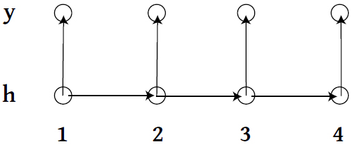
\$\{h_1, h_2, \ldots \} \$ live on discrete space, follow a Markov Process with a transition matrix \$ T_\theta \$.
At time \$ t\$, state \$ h_t \$ emits observation \$ y_t \$ according to some specified model.

AP: first candidate

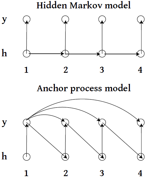
First candidate example

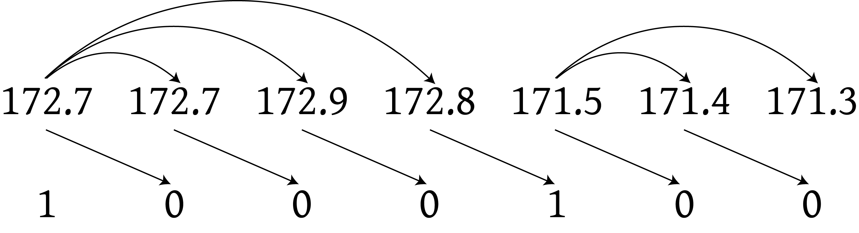
Why would this be a bad candidate?

AP: second candidate

$$$$\begin{align} Y_i \given Y_{r(i)} & \sim N \left(\rho Y_{r(i)} + (1 - \rho) \mu, (1 - \rho^2) \sigma^2 \right), \\Y_i & \sim N\left( \mu, \sigma^2 \right) \rr{ if } r(i)\rr{ doesn't exist}\end{align}$$$$

Needs Gibbs sampler to fit.
Mostly analytic updates.
Needs distributed computing for sensitivity analysis and coverage rate analysis.
Provides good interpretation and interval coverage properties.

Benchmark: coverage

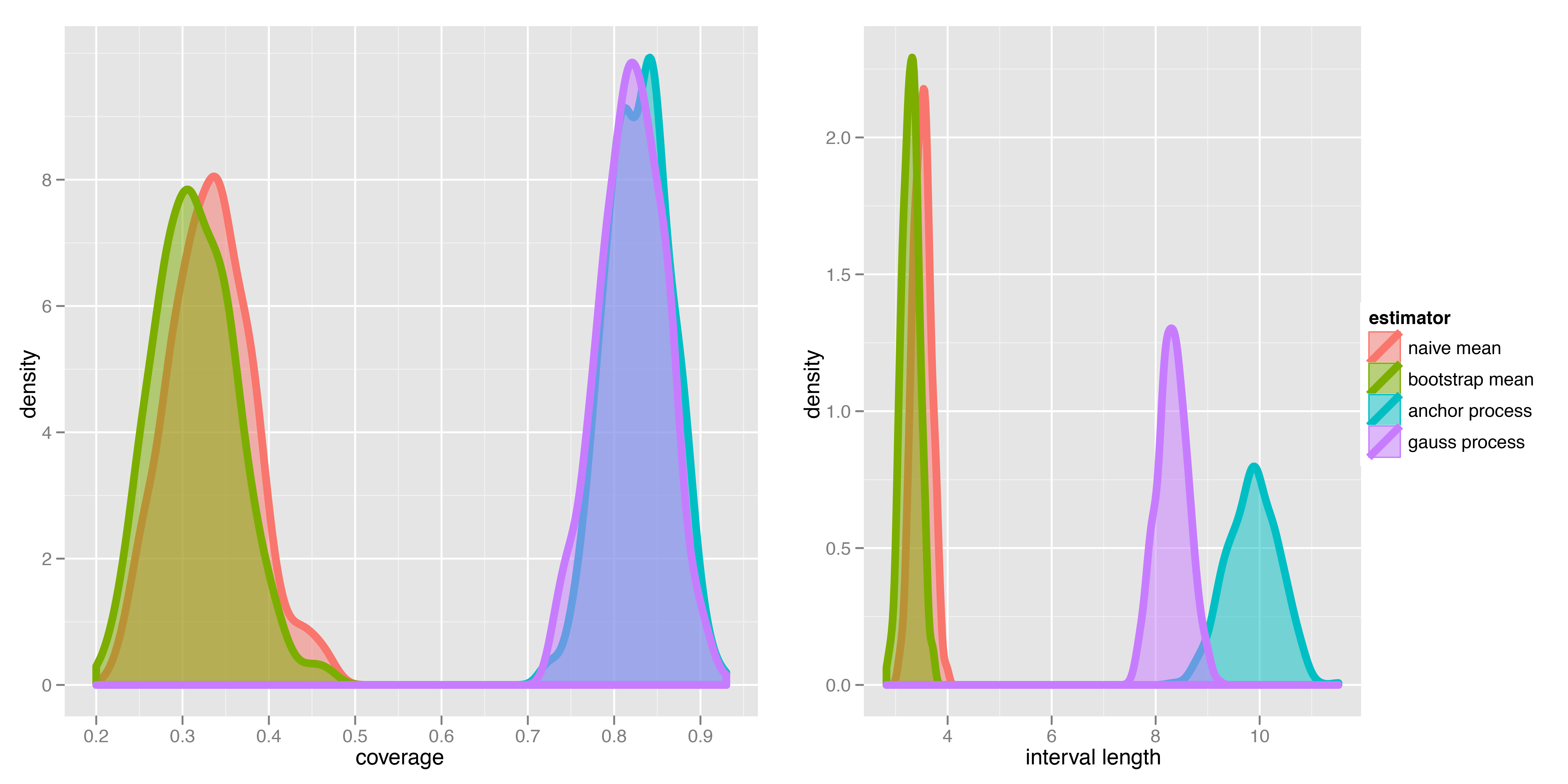
Winner

Second candidate.
Numerically stable (not so many parameters/missing data).
Other favorable features.

What drives the decision?

The estimand.
Model performance metrics.
What models are available/can be adapted?
Work towards parsimony.

Choice of algorithm

Numeric stability.
Cost of implementation and execution.
Point estimation vs. full sampling approaches.
Point estimation: MLE (via LP, QP approximations, EM, Fisher scoring, simulated annealing), MAP.
Full sampling: MCMC, HMC, Gibbs, exact sampling.

Thinking like a programmer

Pseudocode

Simulate from the simple model:

for i in 1:N
  generate and store Y_i from Normal(mu, sigma-sq)

Simulate from the AP model

for i in 1:N
  referrer = r(i)
  if referrer
    Yr = Y_referrer
    generate and store Y_i from Normal(rho * Yr + (1 - rho) * mu, (1 - rho^2) * sigma-sq)
  else
    generate and store Y_i from Normal(mu, sigma-sq)

Pseudocode for main fitting function

initialize parameter values
for i in 1:ndraws
  ## this is Gibbs sampler
  draw mu analytically given current rho and sigma-sq
  draw rho via Metropolis proposals on transformed space given current rho and sigma-sq
  draw sigma-sq analytically given current mu and rho
discard first nburnin draws of parameters

Pseudocode becomes R code

tr = init(data)
for (ii in 1:settings$ndraws) {
  ## this is Gibbs sampler
  pars = lastParams(tr)
  tr$mu = combine(tr$mu, drawMu(data, pars))
  pars = lastParams(tr)
  tr$rho = combine(tr$rho, drawRho(data, pars))
  pars = lastParams(tr)
  tr$ss = combine(tr$ss, drawSigmaS(data, pars))
}
tr = discard(tr, settings$burnin)
tr

Pseudocode becomes good R code

## initialize parameter values
tr = init(data, settings)
## perform the main Gibbs sampler loop
for (ii in 1:settings$ndraws) {
  ## lastParams gets the most recent parameter draws
  pars = lastParams(tr)
  tr$mu = combine(old = tr$mu, add = drawMu(data, pars))
  pars = lastParams(tr)
  tr$rho = combine(old = tr$rho, add = drawRho(data, pars))
  pars = lastParams(tr)
  tr$ss = combine(old = tr$ss, add = drawSigmaS(data, pars))
}
## Burn in - throw away first burnin draws set in settings
tr = discard(allparameters = tr, nthrow = settings$burnin)
tr

Good code

Saves time.
Easier to handle new languages.

Class computing languages

for (ii in 1:10) {
  print("R is awesome")
}

Bash

for ii in $(seq 1 10)
do
  echo "R is awesome"
done

Many code snippets provided in homeworks.

Class visualization languages

Javascript (optional), snippets provided

for (var ii = 0; ii < 10; ii++) {
  console.log("R is awesome");
}

CSS (optional), snippets provided

svg line {
  stroke : #000000;
  opacity : 0.3;
}

HTML (optional), snippets provided

<html>
<body><p>R is awesome</p></body>
</html>

Why need fast code in R

Personal to distributed computing leap.
short_serial, short_parallel queues on Odyssey.
Computing resources are usually constrained.

How to write fast R code

Vectorization.
Think in terms of matrix operations.
Vector indexing.
Built-in functions and functions in packages, some are in lower level languages and so are faster.
(Hint for pset1: may want to consider xpnd in MCMCpack).

Example of fast code in R

time1 <- proc.time()
res1 <- sapply(1:1000000, exp)
time2 <- proc.time()
time2 <- time1
## user system elapsed
## 6.321 0.146 6.429
 
time1 - proc.time()
res2 <- exp(1:1000000)
time2 <- proc.time()
time2 <- time1
## user system elapsed
## 0.022 0.016 0.051
all(res1 == res2)
## [1] TRUE

Problem set 1 visualization

Homework visualization is on the course website.
It's also in the problem set distribution files.

Announcements

Submit your final project rankings by February 10 at noon!
Odyssey access: send your name, email, and phone # to your TF.

Resources

Slides nesterko.com/lectures/stat221-2012/lecture3
Class website theory.info/harvardstat221
Class Piazza piazza.com/class#spring2013/stat221
Class Twitter twitter.com/harvardstat221

Final slide

Next lecture: guest lecture by Rachel Schutt