Expectation-Maximization Algorithm

Stat 221, Lecture 10

@snesterko

Missing Data

Latent variables

Both LV and MD

Does the inference algorithm fully explore the domain, find all modes?
Justification for the selected inference algorithm.
Need more practice (Psets 3-5).

Inference with LV/MD

EM algorithm

Example: ignorant and health aware intentions and running.

For a single person:

$$Z \sim \rr{Beta}(\alpha,\beta), \rr{ } Y_i \given Z \sim \rr{Bernoulli}(Z)$$

Example: likelihood

$$\begin{align}L(\{ \alpha, & \beta\}\given Y, Z) \\ &\propto \prod_{i=1}^n\frac{1}{\rr{B}(\alpha,\beta)}\, z^{y_i + \alpha-1}(1-z)^{1 - y_i + \beta-1}\end{align}$$

The algorithm

Initialize a starting value \$ \theta = \theta^{0}\$.
E step: find \$ Q \$ - the expected value of complete-data log-likelihood given observed data and current values of parameters. $$Q\left( \theta | \theta^{(t)} \right) = \int l(\theta | y) f( Y_{\rr{mis}}| Y_{\rr{obs}}, \theta = \theta^{(t)}) dY_{\rr{mis}}$$
M step: maximize \$ Q \$ with respect to parameters. $$Q \left(\theta^{(t+1)} \given \theta^{(t)}\right) \geq Q\left(\theta \given \theta^{(t)}\right)$$
Iterate between 2 and 3.

Back to example

Main trick is getting the distribution of missing data given observed data and parameters.

$$Z |Y, \alpha, \beta \sim \rr{Beta}\left(\alpha + \sum Y_i, \beta + \sum \left( 1 - Y_i \right) \right)$$

$$E \left( Z \given Y, \alpha, \beta\right) = \frac{\alpha + \sum Y_i}{\alpha + \beta + n}$$

But

The \$ Q \$ function is $$\begin{align}Q = E_{z} & \sum_{i = 1}^n \left[ -\rr{log} \rr{B}(\alpha, \beta) + (y_i + \alpha -1) \rr{log} z \right. \\ & \left. + (1 - y_i + \alpha -1) \rr{log} (1 - z) \right]\end{align}$$

Specifically

$$ \begin{align}Q = & \sum_{i = 1}^n \left[ -\rr{log} \rr{B}(\alpha, \beta) + (y_i + \alpha -1) E_{z}\left(\rr{log} z\right) \right. \\ & \left. + (1 - y_i + \alpha -1) E_z\left(\rr{log} (1 - z)\right) \right]\end{align}$$

Luckily

We know the expected value of the log of a Beta: $$ E_z (\rr{log} Z) = \psi\left(\alpha + \sum Y_i\right) - \psi (\alpha + \beta + n)$$
\$ \psi \$ is the digamma function

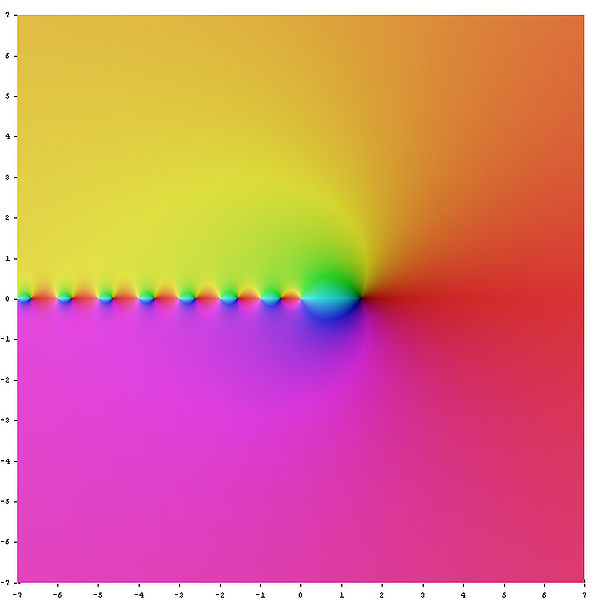
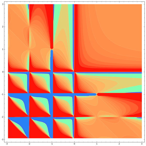
Beta: another pretty function

Algorithm

Set initial values for \$ \alpha, \beta \$.
Calculate \$E_{z}\left(\rr{log} z\right) \$ and \$ E_z\left(\rr{log} (1 - z)\right) \$ given current values of \$ \alpha, \beta \$ and observed data.
Set new values \$ \{ \alpha, \beta\} = \rr{argmax}_{\alpha, \beta} \left[ Q(\alpha, \beta) \right]\$ using the calculated values of \$E_{z}\left(\rr{log} z\right) \$ and \$ E_z\left(\rr{log} (1 - z)\right) \$.
Iterate between 2 and 3 till convergence.

Deriving EM

Relies on Jensen's inequality, and that $$\begin{align}f(Y\given \theta) & = f(Y_{\rr{obs}}, Y_{\rr{mis}} \given \theta) \\ & = f(Y_{\rr{obs}} \given \theta) f(Y_\rr{mis} \given Y_\rr{obs}, \theta)\end{align}$$
Or, by non-negative property of Kullback-Leibler divergence (proved by Jensen's inequality).
Reference: Little and Rubin pp. 172-174.

Some specifics

Complete-data density

$$\begin{align}f(Y\given \theta) & = f(Y_{\rr{obs}}, Y_{\rr{mis}} \given \theta) \\ & = f(Y_{\rr{obs}} \given \theta) f(Y_\rr{mis} \given Y_\rr{obs}, \theta)\end{align}$$

Complete-data log-likelihood

$$\begin{align}l(\theta \given Y) = l(\theta \given Y_{\rr{obs}}) + \rr{log} f(Y_\rr{mis} \given Y_\rr{obs}, \theta)\end{align}$$

Rewrite

$$\begin{align}l(\theta \given Y_{\rr{obs}}) = l(\theta \given Y) - \rr{log} f(Y_\rr{mis} \given Y_\rr{obs}, \theta)\end{align}$$

Take expectation

With respect to \$ Y_\rr{mis} \$ and current estimate \$ \theta^{(t)} \$:

$$\begin{align}l(\theta \given Y_{\rr{obs}}) = Q(\theta \given \theta^{(t)}) - H(\theta \given \theta^{(t)})\end{align}$$

$$\begin{align}Q(\theta | \theta^{(t)}) = \int \left[ l(\theta | Y_{\rr{obs}}, Y_{\rr{mis}})\right]f(Y_{\rr{mis}}| Y_{\rr{obs}}, & \theta^{(t)}) \\ &dY_{\rr{mis}}\end{align}$$

$$\begin{align} H(\theta | \theta^{(t)})= \int & \left[ \rr{log} f(Y_{\rr{mis}}| Y_{\rr{obs}}, \theta^{(t)}) \right] \\ & f(Y_{\rr{mis}}| Y_{\rr{obs}}, \theta^{(t)})dY_{\rr{mis}}\end{align}$$

By Jensen's

$$H \left(\theta \given \theta^{(t)}\right) \leq H \left( \theta^{(t)} \given \theta^{(t)} \right)$$

Also can use the non-negative property of KL divergence (same thing).

Finally

$$\begin{align} l( \theta^{(t+1)} | & Y_{\rr{obs}}) - l( \theta^{(t)} | Y_{\rr{obs}}) = \\ & [Q( \theta^{(t+1)} | Y_{\rr{obs}}) - Q( \theta^{(t)} | Y_{\rr{obs}})] \\ & - [H( \theta^{(t+1)} | Y_{\rr{obs}}) - H( \theta^{(t)} | Y_{\rr{obs}})]\end{align}$$

Since at each iteration of EM we maximize \$ Q \$, the observed-data likelihood must increase.

Fraction of missing info.

Reference: Little and Rubin pp. 177-179.

$$I(\theta \given Y_\rr{obs}) = -D^{20} Q(\theta \given \theta) + D^{20} H( \theta \given \theta)$$

For converged \$ \theta = \theta^* \$, define

$$\begin{align}i_\rr{com} &= \left.-D^{20} Q(\theta \given \theta)\right|_{\theta=\theta^*} \\ i_\rr{obs} & = \left.I(\theta \given Y_\rr{obs})\right|_{\theta=\theta^*} \\ i_\rr{mis} & = \left. -D^{20} H( \theta \given \theta)\right|_{\theta=\theta^*} \end{align}$$

Then have

$$i_\rr{obs} = i_\rr{com} - i_\rr{mis}$$

$$DM = i_\rr{mis}i_\rr{com}^{-1} = I - i_\rr{obs}i_\rr{com}^{-1}$$

\$ DM \$ is the fraction of missing information matrix.

Speed of convergence of EM

Generally, for \$ \theta^{(t)} \$ near \$ \theta^* \$:

$$| \theta^{(t+ 1)} - \theta^* | = \lambda | \theta^{(t)} - \theta^*|$$

where \$ \lambda = DM \$ for scalar \$ \theta \$ and the largest eigenvalue of \$ DM \$ for vector \$ \theta \$.

Dempster, Laird and Rubin (1977)

Ways to "integrate out" missing data

Integrating out the missing data is better, but not always possible. Solutions:

MCMC+
EM+
mcEM
vEM

Essential for computing

Writing the \$ Q \$ function in R vectorization-friendly form.
Implementing vectorized functions.

Example

$$ \begin{align}Q = & \sum_{i = 1}^n \left[ -\rr{log} B(\alpha, \beta) + (y_i + \alpha -1) E_{z}\left(log z\right) \right. \\ & \left. + (1 - y_i + \alpha -1) E_z\left(log (1 - z)\right) \right] = \\ = & n \left[-\rr{log} B(\alpha, \beta) + \left( \bar{y} + \alpha - 1\right)E_{z}\left(log z\right) \right. \\ & \left.+ (1 - \bar{y} + \alpha - 1)E_z\left(log (1 - z)\right) \right]\end{align}$$

Precalculate \$ \bar{ y} \$.

Announcements

T-shirt competitions reminder: it's fun and useful!

Resources

Slides nesterko.com/lectures/stat221-2012/lecture10
Class website theory.info/harvardstat221
Class Piazza piazza.com/class#spring2013/stat221
Class Twitter twitter.com/harvardstat221

Final slide

Next lecture: More on EM, EM for HMM

Case study: research

Alex Franks, non-ignorable missing data mechanism in systems biology.